Discovering Property Valuation
Recently, I discussed the property market with a friend who was a real estate agent. I became fascinated with the real estate market: the marketing, the negotiations, the incentives, and the contracting process. Of greatest interest to me was property valuation. I learned that property sellers used various vendors for valuation, from licensed surveyors to free online tools. Generally, these vendors were not transparent about the techniques they employed, besides stating that these were proprietary. Just for fun, I decided to develop an ML model of my own to explore how ML can be used to value properties.
Existing Valuers
To know how good our model is, we need benchmarks. Here are the main valuers that property sellers go to:
The Singapore Institute of Surveyors and Valuers (SISV)
First, we have the SISV, defined by the Straits Times as "a professional body representing mainly land surveyors, quantity surveyors, valuers, real estate agents and property managers". Its valuers are “licensed under the Appraisers Act”, and must have “a relevant educational background and adequate practical experience”. Therefore, unless you have a Bachelor’s Degree in Real Estate, Property Management, or a similar field, you would not know how exactly your property is being valued, and you would not know how to evaluate the accuracy of the valuation you’re given. In fact, there are no open records of how accurate SISV’s valuations are. Unfortunately, property sellers have high willingness to pay for SISV’s services because SISV is licensed by the government to perform valuations.
Singapore Real Estate Exchange (SRX)
From Wikipedia, SRX is "a consortium of leading real estate agencies administered by StreetSine Technology Group in Singapore". It offers clients several recommended prices, the most famous of which is “X-Value”, a prediction of a property’s value, generated using Comparable Market Analysis (CMA) and property characteristics. See their white paper and statistics on X-Value’s accuracy.
UrbanZoom
UrbanZoom is a property research tool that employs artificial intelligence (AI) to generate accurate property valuations. Their aim is to bring more transparency to the real estate market, because they believe that everyone should be able to buy or sell their homes without any fear of misinformation. UrbanZoom also shares some accuracy statistics on its valuation tool, Zoom Value.
On Transparency
I applaud SRX and UrbanZoom for using modern technical methods to generate valuations, and for openly publishing the accuracy statistics on their predictions. This is a fresh move away from the traditional approach, which employs opaque valuation methods that are protected by legislation. I couldn’t agree more with UrbanZoom’s philosophy, because the negative effects of information asymmetry are amplified in real estate, where each transaction involves hundreds of thousands of dollars. Mispricing a property could mean forgone savings for a child’s university education, or a substantial amount of retirement funds.
In this post, I plan to take transparency one step further by providing a detailed walkthrough of my ML model, which comes close to matching SRX’s X-Value and UrbanZoom’s Zoom Value.
Disclaimer: This post represents only the ML perspective. I used basic ML techniques on open data to generate all findings in this post. I have close to no experience in the property market, and have had no consultations with anyone working in SRX or UrbanZoom.
Executive Summary [TL;DR]
- I modelled the prices of private non-landed and landed properties, and resale HDBs. I called this prediction service “C-Value”.
- C-Value could not beat X-Value’s and Zoom Value’s accuracy, with accuracy measured as the median error and the proportion of predictions within given margins of error.
- C-Value arguably provides a good-enough valuation of private non-landed properties and resale HDBs. Based on the median transaction prices for each property category:
- The error difference (from X-Value / Zoom Value) of 0.04% for private non-landed properties corresponds to $480.
- The error difference of 0.1% for resale HDBs corresponds to $410.
- The error difference of 0.3% for private landed properties corresponds to $9,000.
- The chosen algorithms were:
- Private Non-Landed: K-Nearest Neighbours Regression
- Resale HDB: Gradient Boosting Regression (LightGBM implementation)
- Private Landed: Gradient Boosting Regression (LightGBM implementation)
SRX’s X-Value
SRX uses 4 main metrics to evaluate X-Value: (a) Purchase Price Deviation (PPD), and percentage of price deviations within (b) 5%, (c) 10%, and (d) 20% of X-Value. Metric (a) is simply Transacted Price - X-Value, while the percentage price deviations are computed as ( Transacted Price - X-Value ) / X-Value. To see the statistics for X-Value, see SRX’s webpage here. As shown in the table below, C-Value came close to matching X-Value in generating accurate predictions.
| Private Non-Landed | HDB Resale | Private Landed | ||||
|---|---|---|---|---|---|---|
| Metric | X-Value | C-Value | X-Value | C-Value | X-Value | C-Value |
| Median PPD | 2.7% | 2.74% | 3.1% | 3.2% | 7.7% | 8.0% |
| Within 5% | 70.5% | 69.6% | 70.5% | 69.2% | 36.7% | 34.6% |
| Within 10% | 89.1% | 87.7% | 93.0% | 93.2% | 59.8% | 58.3% |
| Within 20% | 97.7% | 97.3% | 99.2% | 99.7% | 82.8% | 83.2% |
UrbanZoom’s Zoom Value
UrbanZoom provides similar statistics for Zoom Value: (a) Mean Absolute Percentage Error (MAPE) and the percentages of predictions that fell within (a) 5%, (b) 10%, and (c) 20% of actual price. MAPE is computed as ( Zoom Value - Transacted Price ) / Transacted Price. Note that Zoom Value combines predictions for only Condominiums (Private Non-Landed) and resale HDBs. See a comparison of Zoom Value and C-Value in the table below.
| Metric | Zoom Value | C-Value |
|---|---|---|
| Median Error | 3.0% | 3.03% |
| Within 5% | 70% | 69.3% |
| Within 10% | 90% | 91.0% |
| Within 20% | 98% | 98.7% |
Private Non-Landed and Private Landed Property
The Data
The models for private non-landed and landed property were developed using URA caveat data from Aug 2016 to Aug 2019. As you can see in the table below, there were 16 features, including a manual tagging of Non-Landed / Landed under the category feature, and excluding the serial number of each entry.
| S/N | 1 | 2 | 3 |
|---|---|---|---|
| Project Name | WALLICH RESIDENCE | QUEENS | ONE PEARL BANK |
| Street Name | WALLICH STREET | STIRLING ROAD | PEARL BANK |
| Type | Apartment | Condominium | Apartment |
| Postal District | 02 | 03 | 03 |
| Market Segment | CCR | RCR | RCR |
| Tenure | 99 yrs lease commencing from 2011 | 99 yrs lease commencing from 1998 | 99 yrs lease commencing from 2019 |
| Type of Sale | Resale | Resale | New Sale |
| No. of Units | 1 | 1 | 1 |
| Price ($) | 4.3e+06 | 1.55e+06 | 992000 |
| Nett Price ($) | - | - | - |
| Area (Sqft) | 1313 | 1184 | 431 |
| Type of Area | Strata | Strata | Strata |
| Floor Level | 51 to 55 | 26 to 30 | 01 to 05 |
| Unit Price ($psf) | 3274 | 1309 | 2304 |
| Date of Sale | Aug-2019 | Aug-2019 | Aug-2019 |
| category | NonLanded | NonLanded | NonLanded |
Data Cleaning
The data was generally clean, with the exception of the Tenure feature. Here were the key issues and my steps to resolve them:
- Missing entries for
Tenure: Filled in the information using a simple Google search on the relevant properties. - Tenure without start year: I found out that these were properties that were still under construction. I filled in the completion year for these properties through Google.
- Freehold properties had no starting year for tenure: I made the assumption that all Freehold properties were constructed in 1985. On hindsight, this could have affected C-Value’s accuracy.
Feature Engineering
I performed simple feature engineering to extract more value from the dataset. Prior to model training:
- I expanded
Tenureinto three new features to capture more characteristics about the properties:- Remaining Lease
- Age
- Freehold? (binary feature)
- I converted Floor Level into a numeric feature by taking the upper floor within each range. By doing so, we allowed price to be positively correlated to the differences in level between any two given units. On the other hand, one-hot encoding (OHE) would not have allowed us to do this.
- I also converted all non-numeric features into binary features, and dropped unused features like Price, Nett Price, and Date of Sale. The date of sale was dropped because I assumed that there were no major price changes from Aug 2016 to Aug 2019. This may not have been the best assumption.
In model training, I generated a whole set of binary features by applying Term Frequency-Inverse Document Frequency (TF-IDF) to the Project Name and Street Name. Natural Language Processing (NLP) enabled me to make full use of the dataset. In fact, these features turned out to be extremely useful. The intuition behind this was to provide the model with greater fidelity on the properties’ location. The project captured properties in the same development, while the street captured properties in the same neighbourhood. These were created during model training to avoid leakage from incorporating project names and street names that were in the test sets.
Model Training
Features
For both models, I used the same set of features:
- Type*
- Type of Sale*
- Type of Area*
- Market Segment*
- Postal District*
- Age
- Area (Sqft)
- Floor
- Street Name (in binary TF-IDF features)
- Project Name (in binary TF-IDF features)
- Remaining Lease
- Freehold
The features with an asterix were encoded using OHE.
Algorithms
First, I chose K-Nearest Neighbours Regression (K-NN) because the way this algorithm works is extremely similar to how we price properties. In property pricing, we ask “how much did that similar property sell for?” K-NN is effectively the ML implementation of this approach. “Similar” is defined in terms of the features (characteristics of the property) that we put into the model.
Second, I chose Gradient Boosting Regression (LightGBM implementation) simply because it is generally a good algorithm. It is fast, effective, flexible, and can model non-linear relationships.
I did not perform any hyperparameter optimisation for both algorithms in any of the models. This was because I wanted a quick and dirty gauge on how useful ML could be. Only after seeing the models’ results did I see a point in further optimisation.
Evaluation
To evaluate the models, I used 20 repeats of 5-fold cross validation (CV) to generate distributions (n = 100) of each evaluation metric. The metrics were:
- Median Purchase Price Deviation (PPD)
- (Absolute) Price Deviations within 5% of C-Value
- (Absolute) Price Deviations within 10% of C-Value
- (Absolute) Price Deviations within 20% of C-Value
- Mean Absolute Percentage Error (MAPE)
- Mean Absolute Error (MAE)
- R-squared (R2)
- Root Mean Squared Error (RMSE)
I wrote a custom function to run the repeated CV with the following steps for each iteration:
- Create binary TF-IDF features for Project Name and Street Name on the training set and transform the same features in the test set
- Normalise the data if required (only for K-NN)
- Fit a model
- Compute and save metrics
- Go to next iteration and start from Step 1
Model for Private Non-Landed Properties
In the code below, I configured the cross validation object and the data, and ran the K-NN and LightGBM algorithms using my custom function. I reported the mean of the relevant metrics as the final result.
# Configure CV object
cv = RepeatedKFold(n_splits=5, n_repeats=20, random_state=100)

# Configure data
all_vars = ['Type', 'Type of Sale', 'Type of Area', 'Market Segment', 'Postal District', 'age', 'Area (Sqft)', 'floor', 'Street Name', 'Project Name', 'remaining_lease', 'freehold']
dum_vars = ['Type', 'Type of Sale', 'Type of Area', 'Market Segment', 'Postal District']

# Landed data
df_landed = df[df.category == 'NonLanded']

# Configure data
X_data = pd.get_dummies(df_landed[all_vars],
                        columns=dum_vars)
y_data = df_landed['Unit Price ($psf)']

# Run K-NN model
kn = KNeighborsRegressor(n_neighbors=10, weights='distance', n_jobs=4)
kn_cv = custom_cv(kn, X_data, y_data, cv, norm=True, ppd=True)

# Run LightGBM model
lg = LGBMRegressor(n_estimators=500, max_depth=10, random_state=123, n_jobs=4, reg_alpha=0.1, reg_lambda=0.9)
lg_cv = custom_cv(lg, X_data, y_data, cv, norm=False, early=False, ppd=True)
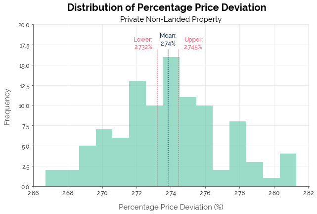
From the results below, we see that K-NN was the better algorithm. However, overall, C-Value did not match up to X-Value across all metrics. Therefore, C-Value is not as robust an ML estimate as X-Value is. However, the difference in median error (0.04%) at the median non-landed price of $1.2M corresponded to a price difference of only $480.
| Metric | X-Value | K-NN | LightGBM |
|---|---|---|---|
| Median PPD | 2.7% | 2.74% | 3.60% |
| Within 5% | 70.5% | 69.61% | 62.57% |
| Within 10% | 89.1% | 87.71% | 85.15% |
| Within 20% | 97.7% | 97.29% | 96.95% |
| MAPE | - | 4.78% | 5.53% |
| MAE | - | $64 | $75 |
| R2 | - | 95.33% | 94.46% |
| RMSE | - | $111 | $121 |
Model for Private Landed Properties
The approach taken was the same as before.
# Configure CV object
cv = RepeatedKFold(n_splits=5, n_repeats=10, random_state=100)

# Configure data
all_vars = ['Type', 'Type of Sale', 'Type of Area', 'Market Segment', 'Postal District', 'age', 'Area (Sqft)', 'floor', 'Street Name', 'Project Name', 'remaining_lease', 'freehold']
dum_vars = ['Type', 'Type of Sale', 'Type of Area', 'Market Segment', 'Postal District']

# Landed data
df_landed = df[df.category == 'Landed']

# Configure data
X_data = pd.get_dummies(df_landed[all_vars],
                        columns=dum_vars)
y_data = df_landed['Unit Price ($psf)']

# Run K-NN model
kn = KNeighborsRegressor(n_neighbors=10, weights='distance', n_jobs=4)
kn_cv = custom_cv(kn, X_data, y_data, cv, norm=True, ppd=True)

# Run LightGBM model
lg = LGBMRegressor(n_estimators=500, max_depth=8, random_state=123, n_jobs=4, reg_alpha=0.1, reg_lambda=0.9)
lg_cv = custom_cv(lg, X_data, y_data, cv, norm=False, early=False, ppd=True)
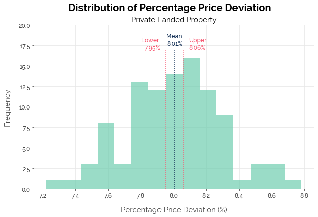
This time, LightGBM was the better algorithm. However, once again, C-Value did not match up to X-Value across all metrics, except in predicting prices within a 20% margin of error. The difference in median error (0.31%) at the median landed price of $3M corresponded to a price difference of $9.3k.
| Metric | X-Value | K-NN | LightGBM |
|---|---|---|---|
| Median PPD | 7.7% | 8.28% | 8.01% |
| Within 5% | 36.7% | 35.86% | 34.64% |
| Within 10% | 59.8% | 55.81% | 58.26% |
| Within 20% | 82.8% | 79.00% | 83.21% |
| MAPE | - | 13.57% | 12.07% |
| MAE | - | $157 | $141 |
| R2 | - | 68.87% | $75.81% |
| RMSE | - | $242 | $213 |
Resale HDBs
The Data
The model for resale HDBs was developed using resale flat price data from HDB, from Jan 2015 to Aug 2019. This dataset comprised 11 features, and we used all of them except the transaction month.
| S/N | 0 | 1 | 2 |
|---|---|---|---|
| month | 2015-01 | 2015-01 | 2015-01 |
| town | ANG MO KIO | ANG MO KIO | ANG MO KIO |
| flat_type | 3 ROOM | 3 ROOM | 3 ROOM |
| block | 174 | 541 | 163 |
| street_name | ANG MO KIO AVE 4 | ANG MO KIO AVE 10 | ANG MO KIO AVE 4 |
| storey_range | 07 TO 09 | 01 TO 03 | 01 TO 03 |
| floor_area_sqm | 60 | 68 | 69 |
| flat_model | Improved | New Generation | New Generation |
| lease_commence_date | 1986 | 1981 | 1980 |
| remaining_lease | 70 | 65 | 64 |
| resale_price | 255000 | 275000 | 285000 |
Data Cleaning
The dataset was extremely clean. I only made three changes:
- Convert
floor areafrom square metres to square feet: This allows us to compare MAE and RMSE with the other models, since they were computed using square feet. - Convert
pricetoprice per square foot (PSF): For alignment with the other models. - Convert
remaining leaseinto years: This was originally included as a string. I simply removed all text except the number of years.
Feature Engineering
Prior to model training, I created the age and floor features, as per the private property dataset. During model training, I applied the same NLP concept for street names (binary TF-IDF to capture more location data).
The one thing I did differently was to generate new features for the units’ block. I separated block numbers from block letters, and created binary features for each block number and letter. The idea here was to add more location information. Flats previously sold within the same block should have some influence on the price of any given flat in that block.
Model Training
Algorithms and Evaluation
I used the same approach as before.
Model for Resale HDBs
# Configure CV object
cv = RepeatedKFold(n_splits=5, n_repeats=10, random_state=100)

# Read data
resale = pd.read_csv('HDB/resale_final.csv')

# FE for blocks
resale['block_num'] = resale.block.str.replace('[A-Z]', '')
resale['block_letter'] = resale.block.str.replace('[0-9]', '')
resale = resale.drop('block', axis=1)

# Configure features
hdb_vars = ['town', 'flat_type', 'block_num', 'block_letter', 'street_name', 'sqft', 'flat_model', 'remaining_lease', 'price', 'age', 'floor']
hdb_dum_vars = ['town', 'flat_type', 'flat_model', 'block_num', 'block_letter']

# Configure data
X_data = pd.get_dummies(resale[hdb_vars],
                        columns=hdb_dum_vars).drop('price', axis=1)
y_data = resale['price']

# Run K-NN model
kn = KNeighborsRegressor(n_neighbors=15, weights='distance', n_jobs=4)
kn_cv = custom_cv(kn, X_data, y_data, cv, norm=True, ppd=True)

# Run LightGBM model
lg = LGBMRegressor(n_estimators=5000, max_depth=25, random_state=123, n_jobs=4, reg_alpha=0.1, reg_lambda=0.9)
lg_cv = custom_cv(lg, X_data, y_data, cv, norm=False, early=False, ppd=True)
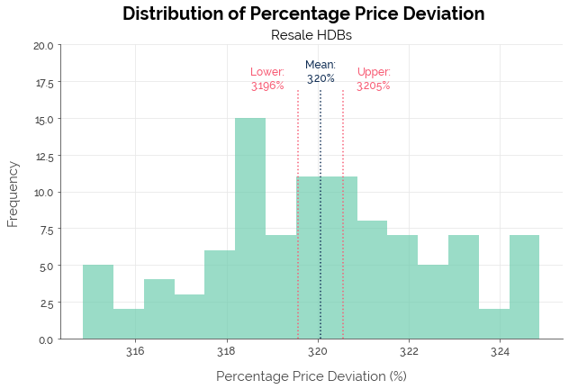
Once again, LightGBM was the better algorithm. Yet, C-Value fared worse than X-Value in (1) the median error and in (2) predicting prices within a 5% margin of error. The difference in median error (0.1%) at the median resale HDB price of $410k corresponded to a price difference of only $410.
| Metric | X-Value | K-NN | LightGBM |
|---|---|---|---|
| Median PPD | 3.1% | 3.93% | 3.20% |
| Within 5% | 70.5% | 60.04% | 69.14% |
| Within 10% | 93.0% | 87.73% | 93.27% |
| Within 20% | 99.2% | 99.19% | 99.72% |
| MAPE | - | 5.08% | 4.12% |
| MAE | - | $21 | $17 |
| R2 | - | 92.87% | 95.29% |
| RMSE | - | $29 | $23 |
Zoom Value: Private Non-Landed and Resale HDBs
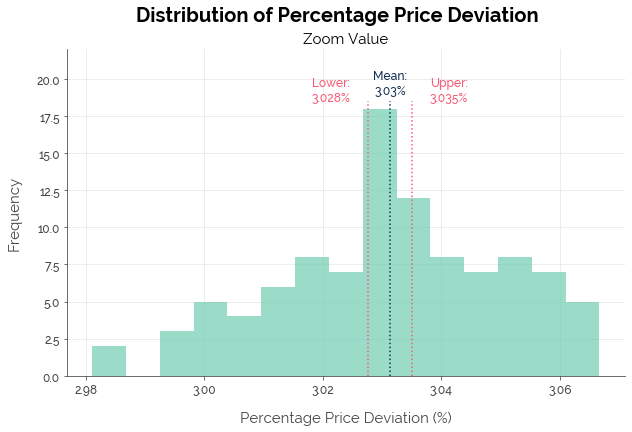
I combined the best models for private non-landed properties (K-NN) and resale HDBs (LightGBM) to create the C-Value equivalent to Zoom Value. Overall, C-Value couldn’t match Zoom Value in terms of the median error and the proportion of predictions within 5% accuracy. There was no comparable price difference resulting from the difference in median error, because UrbanZoom did not break down the accuracy statistics by the type of property.
| Metric | Zoom Value | C-Value |
|---|---|---|
| Median Error | 3% | 3.03% |
| Within 5% | 70% | 69.33% |
| Within 10% | 90% | 91.02% |
| Within 20% | 98% | 98.74% |
Improving the Model
Although the dollar price differences due to the median error differences were small, C-Value failed to beat X-Value and Zoom Value in terms of hard ML performance metrics. Here are some possible reasons why:
- Too little data. The models were trained on relatively recent data, as opposed to a large bank of data on housing prices. The good thing about this approach is that it avoids using old data that may have become irrelevant. The tradeoff is that some of the older data could be useful. For example, 5 years could have been an acceptable time frame for the dataset.
- No temporal effects. The models assumed that relationships in the data were stable during the time frames in the respective dataset. However, one month’s prices could be related to the following month’s prices. Including temporal features like lagged prices for a given type of property could improve prediction.
- Simple algorithms. K-NN was a good model because it accurately models business thinking on valuation, and LightGBM is a good model in general. However, other sophisticated approaches could have been tested. For example, stacked regression can be used to control outlying predictions and thereby improve MAPE.
Conclusion
In this post, I showed that basic ML algorithms could produce acceptable valuations (C-Value) of Singapore properties. Although these could not match up to the predictive accuracy of X-Value and Zoom Value in terms of median error and the proportion of predictions within given margins of error, these were good enough for providing a rough estimate of value.
More generally, I showed that there is value in using ML for quantifying relationships between characteristics of a property (and/or its similar properties) and its market price. This also means that ML can be used to quantify and recommend a fair listing price. This would be an alternative to SRX’s X-Listing Price, the only all-in-one recommendation service provided to sellers that is available on the market. I’ll save this for next time :)
Credits for image: Nanalyze