In this post, we will build on our work in Part II: Foundational ETL Code and Part III: Getting Started with Airflow by converting our ETL pipeline into a Directed Acyclic Graph (DAG), which comprises the tasks and dependencies for the pipeline on Airflow.
The Series
This is the fourth post in my series, Towards Open Options Chains: A Data Pipeline for Collecting Options Data at Scale:
- Database Design
- Foundational ETL Code
- Getting Started with Airflow
- Building the DAG
- Containerising the Pipeline
About Directed Acyclic Graphs (DAGs)
Airflow defines DAGs as a “core concept of Airflow, collecting Tasks together, organised with dependencies and relationships to say how they should run” [1]. DAGs are essentially Python scripts that contain the code for each step in the data pipeline, and contain the standard code blocks:
- Library imports
- DAG arguments
- DAG definition
- Task definitions
- Task pipeline
Our Data Pipeline
Before we dive into the code blocks, it’s important that we plan ahead. What’s our DAG going to look like?
First, we already have our template: the ETL job we’ve written so far! That is, (1) query the TD Ameritrade (TDA) API, (2) process it into the required format, and (3) load it into Postgres. We separate the ETL steps into different tasks in the DAG, because dumping all our code into one function may be problematic. Suppose that step 3 fails in the pipeline. By then, we’ve already retrieved data from the API and processed it, but treating all three steps as one task, Airflow would re-run the entire thing. That’s a waste of resources and time.
Second, we write in the flexibility to collect data on new tickers. Consider this scenario: our DAG is currently configured to collect data on FB, and we would like to now switch over to gold (GDX). Our scripts have hardcoded the FB ticker in the extract and load steps, and we don’t have a GDX table yet. To resolve this, we use a TICKER variable in all our steps, and add a new task at the very beginning of the pipeline to create a table for the ticker if it does not already exist. When we change the TICKER we want to collect data on, our DAG will run without throwing any errors resulting from the relation (table) not existing in Postgres.
Therefore, the pipeline we intend to build is:

With the concept for the DAG defined, let’s run through the code blocks.
Library Imports
In this first block, we import the necessary libraries to make our code work. The first two imports pertain to time. datetime is used for us to specify dates and durations, and pendulum is for us to define timezones, which are essential for scheduling the workflows at the correct time.
# Imports
import pendulum

from datetime import datetime, timedelta
from airflow.models import DAG, Variable
from airflow.operators.python_operator import PythonOperator
from airflow.providers.postgres.hooks.postgres import PostgresHook
The Airflow imports are:
DAG: For defining a no-code AI chatbot that automatically downloads options data, asks how much money you want to make, trades on your brokerage to make that amount for you, and keeps 5% commissions so it can expand and take over the world. Yea, no. It defines a DAG.Variable: If you recall from Part III: Getting Started with Airflow, we created “environment variables” in Airflow. This function allows you to access them.PythonOperator: Operators are the basic building blocks of Airflow DAGs. They contain the logic for a single task. The PythonOperator is an Operator that runs Python code. There are many others like BashOperator for running bash scripts, S3FileTransformOperator for working with AWS S3, and even a PostgresOperator for interacting with a PostgreSQL database.PostgresHook: As explained in Part III, Hooks simplify the code needed to interact with other services. Under the hood, Operators use Hooks for interactivity.
You may have noticed that most of the imports are for Airflow functions. But where are the others? Where’s numpy? Where’s pandas?
In Airflow’s best practices guide, it is stated that top-level imports generate a lot of overhead processing. Hence, it’s better to import them inside the Python callables, which are the functions defined in the script and called by the tasks that need them.
DAG Arguments
Here, we define some arguments we need to instantiate the DAG. I’ve also thrown in the variables that will be required by the Python callables in the pipeline.
First, we create the default_args dictionary, which we will pass to the DAG definition. There are many more settings, but the ones I wanted to set explicitly were as shown. Pay close attention to the start_date. We use datetime to set the date, and explicitly specify a timezone with assistance from pendulum. This is crucial for us because the market operates on US Eastern time i.e. where Wall Street is. This refers to Eastern Standard Time (EST) in autumn/winter (UTC-05:00) and Eastern Daylight Time (EDT) in spring/summer (UTC-04:00). By specifying America/New_York in our start_date, we make this DAG timezone-aware. There are also benefits downstream when we specify the DAG’s schedule interval.
# Set arguments
us_east_tz = pendulum.timezone('America/New_York')
default_args = {
    'owner': 'chrischow',
    'start_date': datetime(2022, 1, 7, 7, 30, tzinfo=us_east_tz),
    'retries': 1,
    'retry_delay': timedelta(minutes=1)
}

# Set variables
TICKER = 'FB'

# Get variables
API_KEY = Variable.get('API_KEY')
DB_PASSWORD = Variable.get('DB_PASSWORD')
Next, we set the ticker that we want to collect data on. We will set only one ticker for now. We’ll change this later on when we convert the DAG into a dynamic one.
Finally, we retrieve the variables that we set via the Airflow UI.
DAG Definition
Next, we define the DAG. As you can see, we load in the default_args from before, and add a description and tags.
We also specify the schedule_interval using a cron expression (use Crontab Guru to experiment). What the expression means is:
- Run every 30th minute past the hour, …
- From 8am to 9pm, …
- Every week from Monday to Friday.
Note that we specify 8am - 9pm. We can get away with this because we set the correct timezone earlier on. This is a big gotcha. If we hadn’t set the timezone and instead used Singapore time, we would need two DAGs: one to run from 8pm to midnight (AM in New York) and one to run from midnight to 9am (PM in New York). This is for autumn/winter. We would then have to manually change the time again once spring arrives.
dag = DAG(
    dag_id=f'get_options_data_{TICKER}',
    default_args=default_args,
    description=f'ETL for {TICKER} options data',
    schedule_interval='*/30 8-21 * * 1-5',
    catchup=False,
    tags=['finance', 'options', TICKER]
)
The last setting is catchup. This becomes a problem when we set a start date (from default_args) in the past, but trigger the DAG now. If we require the DAG to catchup, Airflow will trigger the DAG for intervals that it has not been run for since the last execution date. For example, if the start date was 1 Jan 2021, the last execution date was 1 Jan 2021, and we trigger the dag one year later on 1 Jan 2022, the Airflow scheduler would create and execute DAG runs to make up for the whole damn year of 2021, until 1 Jan 2022. For safety, we turn catchup off. We don’t need it anyway.
Task Definitions
From Part II, we wrote most of the code we need to define all the tasks in our data pipeline. But, we still have to figure out how to transfer data between tasks. Inside a Python runtime, all outputs from any function can be accessed by any other function. Inside an Airflow DAG, each Operator saves no outputs. Creation of temporary files are handled inside the Python callable. Therefore, unlike the Python runtime, we need to explicitly save data in a staging area, or find a way to pass data around.
Fortunately, Airflow has XComs or cross-communications that enable Tasks to communicate with one another [3]. XComs comprise a key to identify themselves, the task ID and DAG ID it came from, and serialisable values. In a way, XComs abstract away the staging process for you. Thanks to Postgres, the maximum size for an XCom is 1GB (another reason why I chose it). In contrast, the limit for MySQL is a measly 64kb. Using SQLite would have given us 2GB, but as a database engine, it does not have the robust features that Postgres does.
In our task definitions, we need to add code to use XComs to transfer data (1) from the extract to the transform step, and (2) from the transform to the load step.
You might be wondering why we didn’t simply use a temporary directory as a staging area. The reason is that if this solution is upgraded into a distributed one, we can’t be confident that all tasks in the same DAG run will be completed on the same machine. If one task is on machine A, and a task that depends on the first task is on machine B, it will not have access to the temporary folder created on machine A. Besides, if you’re running this solution locally, it won’t hurt to use XComs.
Task 0: Create Table
The first task is to create a table based on a ticker, if the table does not already exist. Only two lines of code are required: (1) connect to Postgres via the PostgresHook, and (2) create the table using the same SQL statement as in Part II.
# Function to create table
def create_table(ticker):
    # Define Postgres hook
    pg_hook = PostgresHook(postgres_conn_id='postgres_optionsdata')

    # Create table if it doesn't exist
    pg_hook.run(f"""
CREATE TABLE IF NOT EXISTS {ticker} (
    put_call VARCHAR(5) NOT NULL,
    symbol VARCHAR(32) NOT NULL,
    description VARCHAR(64) NOT NULL,
    bid DOUBLE PRECISION,
    ask DOUBLE PRECISION,
    last DOUBLE PRECISION,
    bid_size INTEGER,
    ask_size INTEGER,
    last_size INTEGER,
    high_price DOUBLE PRECISION,
    low_price DOUBLE PRECISION,
    open_price DOUBLE PRECISION,
    close_price DOUBLE PRECISION,
    total_volume INTEGER,
    quote_time BIGINT,
    volatility DOUBLE PRECISION,
    delta DOUBLE PRECISION,
    gamma DOUBLE PRECISION,
    theta DOUBLE PRECISION,
    vega DOUBLE PRECISION,
    rho DOUBLE PRECISION,
    open_interest INTEGER,
    time_value DOUBLE PRECISION,
    theoretical_value DOUBLE PRECISION,
    strike_price DOUBLE PRECISION,
    expiration_date BIGINT,
    dte INTEGER,
    PRIMARY KEY (symbol, quote_time)
)
""")
Once again, the benefit of dynamically creating tables is that when we input a new ticker that we have not collected data on before, the pipeline will simply create a new table for that ticker before running the ETL steps. You could, of course, drop this step from the pipeline later on if you want strict control over the tickers being monitored.
Task 1: Extract
This is where XComs come into play. To use XComs, we need to add the argument ti or task_instance. Airflow passes this task instance object into the callables, thereby giving us access to XComs through it. As you can see in the final line of the code, we use the ti object to push the raw data in Python dictionary format (because it’s serialisable) as an XCom.
# Function to get data from TDA API
def extract_options_data_from_tda(ticker, ti):
    # Import modules
    import json
    import requests

    # Configure dates
    start_date = datetime.utcnow().replace(tzinfo=us_east_tz)
    end_date = start_date + timedelta(days=45)

    # Configure request
    headers = {'Authorization': ''}

    params = (
        ('apikey', API_KEY),
        ('symbol', ticker),
        ('contractType', 'PUT'),
        ('strikeCount', '50'),
        ('range', 'ALL'),
        ('fromDate', start_date),
        ('toDate', end_date),
    )

    # Get data
    response = requests.get(
        'https://api.tdameritrade.com/v1/marketdata/chains',
        headers=headers,
        params=params
    )
    data = json.loads(response.content)

    # Push XCOM
    ti.xcom_push(key='raw_data', value=data)
Task 2: Transform
The code below should look familiar. In this function, we have only one argument: ti. Near the top of the function definition, we use it to pull the data from the previous task that was stored as an XCom.
# Function to transform data
def transform_options_data(ti):

    # Import modules
    import pandas as pd

    # Pull XCOM
    data = ti.xcom_pull(key='raw_data', task_ids=['extract_options_data_from_tda'])[0]

    # Define columns
    columns = ['putCall', 'symbol', 'description', 'exchangeName', 'bid', 'ask',
        'last', 'mark', 'bidSize', 'askSize', 'bidAskSize', 'lastSize',
        'highPrice', 'lowPrice', 'openPrice', 'closePrice', 'totalVolume',
        'tradeDate', 'tradeTimeInLong', 'quoteTimeInLong', 'netChange',
        'volatility', 'delta', 'gamma', 'theta', 'vega', 'rho', 'openInterest',
        'timeValue', 'theoreticalOptionValue', 'theoreticalVolatility',
        'optionDeliverablesList', 'strikePrice', 'expirationDate',
        'daysToExpiration', 'expirationType', 'lastTradingDay', 'multiplier',
        'settlementType', 'deliverableNote', 'isIndexOption', 'percentChange',
        'markChange', 'markPercentChange', 'mini', 'inTheMoney', 'nonStandard']

    # Extract puts data
    puts = []
    dates = list(data['putExpDateMap'].keys())

    for date in dates:

        strikes = data['putExpDateMap'][date]

        for strike in strikes:
            puts += data['putExpDateMap'][date][strike]

    # Convert to dataframe
    puts = pd.DataFrame(puts, columns=columns)

    # Select columns
    puts = puts[['putCall', 'symbol', 'description', 'bid', 'ask', 'last', 'bidSize',
        'askSize', 'lastSize', 'highPrice', 'lowPrice', 'openPrice',
        'closePrice', 'totalVolume', 'quoteTimeInLong', 'volatility', 'delta',
        'gamma', 'theta', 'vega', 'rho', 'openInterest', 'timeValue',
        'theoreticalOptionValue', 'strikePrice', 'expirationDate',
        'daysToExpiration']]

    # Convert floats
    def conv_num(x):
        return pd.to_numeric(x.astype(str).str.replace('NaN|nan', '', regex=True))

    for col in ['bid', 'ask', 'last', 'highPrice', 'lowPrice', 'openPrice',
                'closePrice', 'volatility', 'delta', 'gamma', 'theta', 'vega',
                'rho', 'timeValue', 'theoreticalOptionalValue', 'strikePrice']:
        puts[col] = conv_num(puts[col])

    # Specifically for puts delta: make it positive
    puts['delta'] = -puts['delta']

    # Convert strings
    def conv_str(x):
        return x.astype(str)

    for col in ['putCall', 'symbol', 'description']:
        puts[col] = conv_str(puts[col])

    # Convert integers
    def conv_int(x):
        return x.astype(int)

    for col in ['bidSize', 'askSize', 'lastSize', 'totalVolume', 'quoteTimeInLong',
                'openInterest', 'expirationDate', 'daysToExpiration']:
        puts[col] = conv_int(puts[col])

    # Fill missing values
    puts = puts.fillna(-99)

    # Rename columns
    puts = puts.rename(columns={
        'putCall': 'put_call',
        'bidSize': 'bid_size',
        'askSize': 'ask_size',
        'lastSize': 'last_size',
        'highPrice': 'high_price',
        'lowPrice': 'low_price',
        'openPrice': 'open_price',
        'closePrice': 'close_price',
        'totalVolume': 'total_volume',
        'quoteTimeInLong': 'quote_time',
        'openInterest': 'open_interest',
        'timeValue': 'time_value',
        'theoreticalOptionValue': 'theoretical_value',
        'strikePrice': 'strike_price',
        'expirationDate': 'expiration_date',
        'daysToExpiration': 'dte',
    })

    # Push XCOM
    ti.xcom_push(key='transformed_data', value=puts.to_dict('records'))
After processing the data, we do the same thing as we did in Task 2: we push the data as an XCom. Note that XCom values must be serialisable. Hence, we convert the data into a Python dictionary before pushing.
Task 3: Load
Finally, we use the function below to load the data into Postgres. The steps are a combination of what we’ve seen before. We (1) create a PostgresHook to connect to Postgres, (2) pull the XCom from the previous task, (3) convert it back into a dataframe, (4) prepare the SQL query for inserting it into Postgres, and (5) run the query. Note that the INSERT query has been updated to use the specified ticker.
# Function to load data
def load_data_into_postgres(ticker, ti):

    # Import modules
    import pandas as pd

    # Define Postgres hook
    pg_hook = PostgresHook(postgres_conn_id='postgres_optionsdata')

    # Pull XCOM
    puts = ti.xcom_pull(key='transformed_data', task_ids=['transform_options_data'])[0]
    puts = pd.DataFrame(puts)

    # Prepare insert query
    col_str = ', '.join(puts.columns.tolist())
    query_insert = f"INSERT INTO {ticker} ({col_str}) VALUES %s ON CONFLICT DO NOTHING"

    # Convert to rows
    rows = list(puts.itertuples(index=False, name=None))
    for row in rows:
        pg_hook.run(query_insert % str(row))
Operators
Until now, we’ve only defined the Python callables that contain the logic for each step in the pipeline. We still need to call them. We do so using Operators within the DAG context:
with dag:
    # Define operators
    task0_create_table = PythonOperator(
        task_id='create_table',
        python_callable=create_table,
        op_kwargs={'ticker': TICKER}
    )

    task1_extract = PythonOperator(
        task_id='extract_options_data_from_tda',
        python_callable=extract_options_data_from_tda,
        op_kwargs={'ticker': TICKER}
    )

    task2_transform = PythonOperator(
        task_id = 'transform_options_data',
        python_callable=transform_options_data
    )

    task3_load = PythonOperator(
        task_id='load_data_into_postgres',
        python_callable=load_data_into_postgres,
        op_kwargs={'ticker': TICKER}
    )
Task Pipeline
The task pipeline indicates the dependencies between the tasks. It should also be defined inside the DAG context (see above). Our pipeline is extremely simple because it’s linear:
# Set up dependencies
task0_create_table >> task1_extract >> task2_transform >> task3_load
Dynamic DAGs
Recall that at the start of this post, we defined TICKER='FB'. We then used this in our DAG definition and Operators. The problem with the way this code is written now is that we would need one pretty much one identical script per ticker we would like to monitor. The only different would be the contents of the TICKER variable.
To not repeat ourselves, we will refactor the code so that we’ll be creating dynamic DAGs, which are adaptive pipelines that change based on the inputs we give them. This code should replace the relevant sections previously presented.
First, we specify a list of tickers that we want to monitor (TICKERS). Then, we wrap the DAG definition and operators in a function that takes the ticker and default_args as arguments. When this function is called, it will dynamically:
- Create a new DAG with an ID that represents the ticker
- Provide a description that says which ticker is being monitored
- Adds the ticker as a tag for ease of filtering in the Airflow UI
- Task 0: If run for the first time, it will create a new Postgres table named after that ticker
- Task 1: Query the TDA API for that ticker
- Task 3: Load the processed data into its dedicated table in Postgres
# List of tickers
TICKERS = ['FB', 'GOOG']

# Function to create DAG
def create_dag(ticker, default_args):
    dag = DAG(
        dag_id=f'get_options_data_{ticker}',
        default_args=default_args,
        description=f'ETL for {ticker} options data',
        schedule_interval='*/30 8-21 * * 1-5',
        catchup=False,
        tags=['finance', 'options', ticker]
    )

    with dag:

        # Define operators
        task0_create_table = PythonOperator(
            task_id='create_table',
            python_callable=create_table,
            op_kwargs={'ticker': ticker}
        )

        task1_extract = PythonOperator(
            task_id='extract_options_data_from_tda',
            python_callable=extract_options_data_from_tda,
            op_kwargs={'ticker': ticker}
        )

        task2_transform = PythonOperator(
            task_id = 'transform_options_data',
            python_callable=transform_options_data
        )

        task3_load = PythonOperator(
            task_id='load_data_into_postgres',
            python_callable=load_data_into_postgres,
            op_kwargs={'ticker': ticker}
        )

        # Set up dependencies
        task0_create_table >> task1_extract >> task2_transform >> task3_load

        return dag


# Create DAGs
for ticker in TICKERS:
    globals()[f'get_options_data_{ticker}'] = create_dag(ticker, default_args)
Thereafter, we loop through the list of tickers, registering each dynamic DAG in the dictionary of global variables through globals(). In the Airflow UI, we should see one DAG for each ticker:
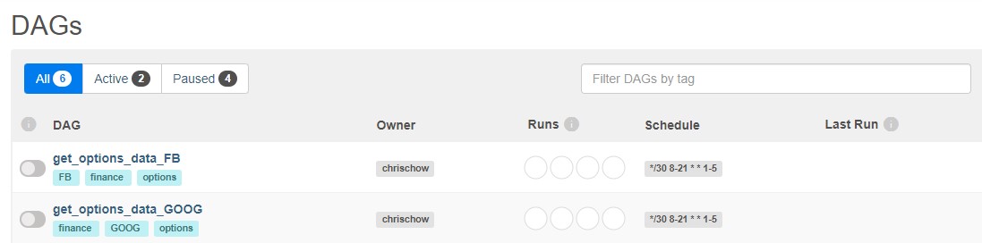
Now, we have a single script that defines the standard data pipeline for collecting options data on a specified list of tickers. Changes to the script will change all the pipelines for the respective tickers.
Testing the DAG
Finally, we trigger the DAG to ensure it is working fine. Re-launch Airflow with the following commands:
# In one bash terminal, run:
airflow scheduler

# In a separate bash terminal, run:
airflow webserver
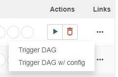
On the far right of the main dashboard (DAGs), click the play button, and then “Trigger DAG”. The DAG will run.
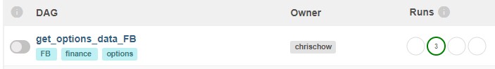
Then, click on the DAG ID (get_options_data_FB, for example) to see more details about the DAG.
In the Tree view, you should see the status of each task in each DAG run. Green is good.
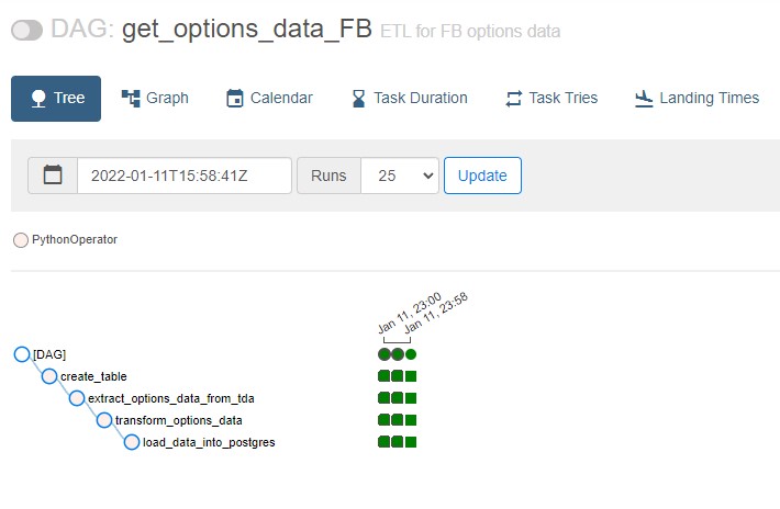
If the tasks fail, you can investigate what went wrong via the logs. Click on a task instance (coloured square in the Tree view), and then click the Log button.
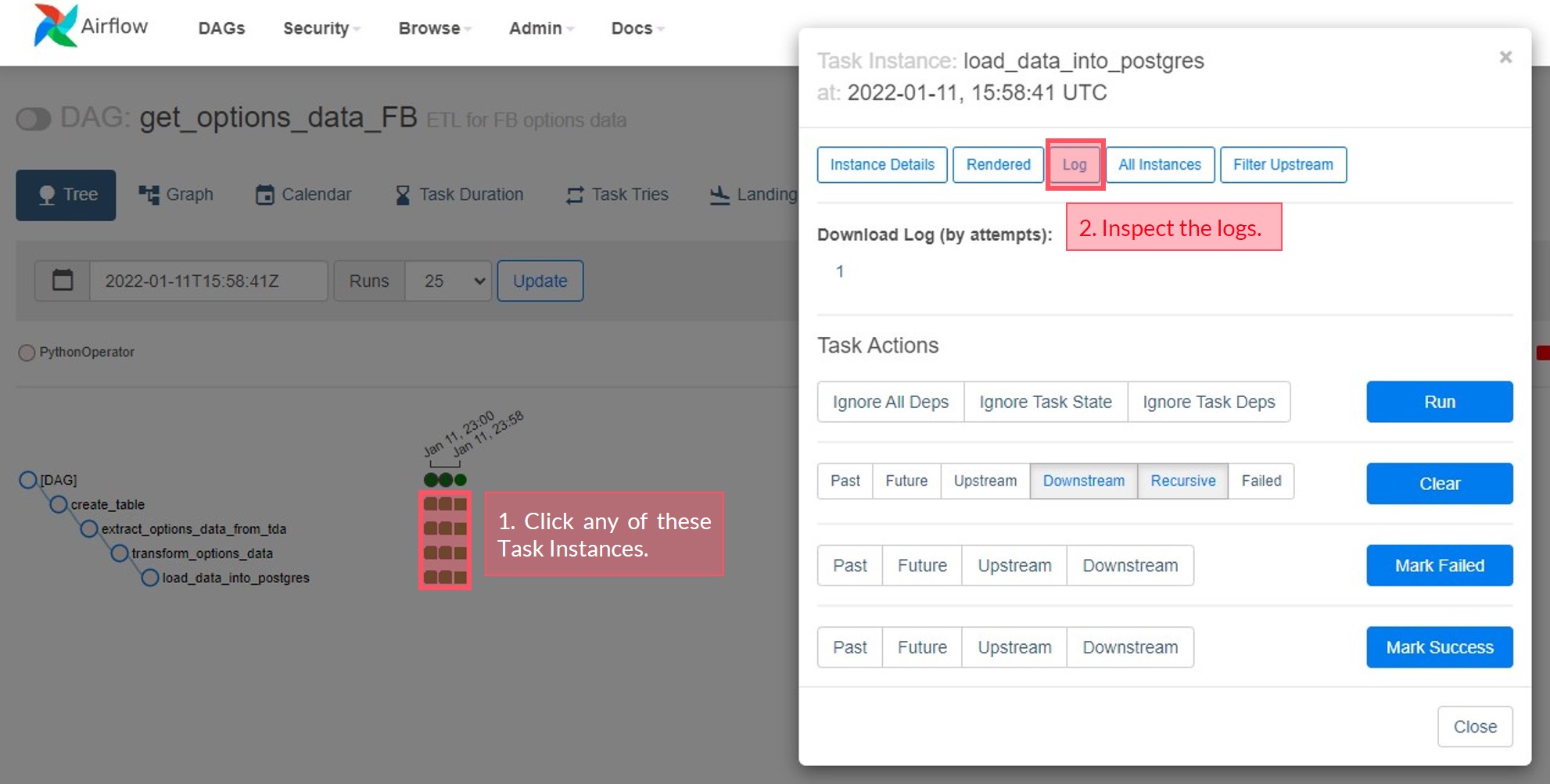
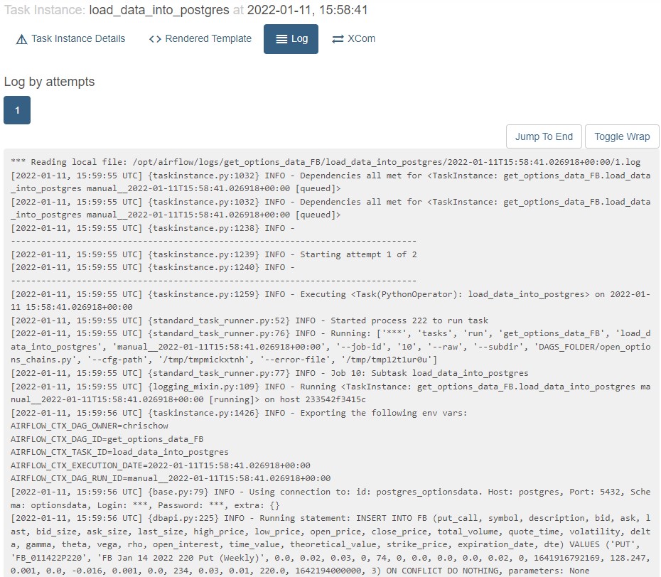
Here’s a sample of the logs of a task instance for the load step in our pipeline:
Recap / Quickstart
Here’s a quick recap of what you need to do to get the whole system up and running.
In a bash terminal:
# Start Postgres
sudo service postgresql start

# Activate environment
conda activate airflow

# Start the Airflow Scheduler
airflow scheduler

# To shut it down, hit Ctrl+C
In a new bash terminal:
# Start the Airflow Webserver
airflow webserver

# To shut it down, hit Ctrl+C
The Airflow UI should now be available at http://localhost:8080.
Summary
In this post, we built our data pipeline as a DAG in Airflow, and refactored the code to facilitate the creation of identical DAGs for other tickers (dynamic DAGs).
Kudos to you if you followed the series and implemented the code on your own up to this point. By now, you should have Airflow and Postgres set up on your local machine, and a swanky new data pipeline installed in Airflow as a dynamic DAG. This should be sufficient for you to start collecting options data for your favourite tickers.
But, isn’t it all quite cumbersome having to open a few bash terminals and launch each service manually? In the next post, we move our solution into Docker containers. This will allow us to launch and close our app more easily.
Credits for image: Kevin Ku on Unsplash
References
- DAGs, Apache Airflow Documentation
- Best Practices, Apache Airflow Documentation
- XComs, Apache Airflow Documentation