Part I: Designing the Database
Since September last year, I started trading options. Naturally, I wanted to use data to validate my strategies. But, it was tough getting hold of intra-day options data. I was surprised to learn that it is expensive as hell: a subscription for 30-minute data (quotes and greeks) for 10 tickers costs about USD400 per month. While there are free options quotes, there are no open databases. Hence, I decided to develop the means to build one.
Why Read On?
Getting free options data isn’t exactly a new problem. Others have developed different methods (at the time of writing) that primarily involve scraping and processing data (see table below). These are well and good if you prefer having the flexibility to adapt the provided code, schedule them to run at the required intervals, and develop custom logging features for the entire process on your own.
| Implementation | Source | Destination | Source |
|---|---|---|---|
| One-off Python script | Ally Financial API | SQLite DB | Eric Kleppen on TowardsDataScience [1] |
| One-off Python script | Barchart.com | HDFS | Blackarbs [2] |
| Python script with some scheduling capability | Yahoo Finance | CSV file | Harry Sauers on freeCodeCamp [3] |
| One-off Python script | Yahoo Finance (through yahoo_fin package) |
Python dictionary | Andrew Treadway on TheAutomatic.net [4] |
| One-off Python script | Yahoo Finance (through yfinance package) |
Pandas dataframe | Tony Lian on TowardsDataScience [5] |
| One-off Python script | Yahoo Finance (through pandas_datareader package) |
Pandas dataframe | CodeArmo [6] |
| One-off Python script | Yahoo Finance (through yfinance package) |
Pandas dataframe | Ran Aroussi [7] |
| Data pipeline run at scheduled intervals through Apache Airflow | TD Ameritrade API | PostgreSQL | Me! |
A more holistic approach would automate those things for you. And that is the contribution of this series: I develop a data pipeline to extract data from a different source - the TD Ameritrade (TDA) API - process the data, and persist it in a PostgreSQL database, using Apache Airflow to define, schedule, and monitor the entire workflow.
In this post, we discuss the requirements for solutions on different scales (based on the number of stocks to collect data on), and design our database.
The Series
This is the first post in my series, Towards Open Options Chains: A Data Pipeline for Collecting Options Data at Scale:
- Designing the Database
- Foundational ETL Code
- Getting Started with Airflow
- Building the DAG
- Containerising the Pipeline
The Use Case
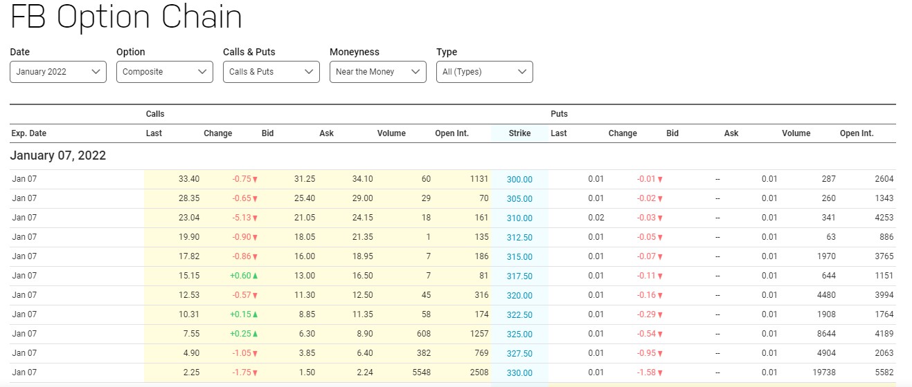
The use case for the data is fairly straightforward: to run backtests of options trading strategies. Therefore, the data pipeline must collect sufficiently fine-grained data. We will need options prices, volumes, and the options greeks (e.g. delta, theta, and gamma), collected at sufficiently high frequency. In case you’ve never seen options data before, see the screenshot below for a sample.
While I only intend to run this on a limited set of 10-20 stocks, we have to consider that some users out there may use this solution for collecting data on a huge scale, say 1,000 stocks. We assume that the small scale scenario (20 stocks) is for individual use by retail investors, and the large scale scenario (1,000 stocks) is for serving the data to a wider group of users. In designing the solution, we focus on the small scale scenario, but keep the large scale scenario in mind.
Examining the Data
Before we go about designing the database, it would be helpful to inspect a sample of the data. Fortunately, we can do this because the TDA Option Chains API is readily available. We will skip over the steps to obtain credentials and the code to retrieve the data for now.
Data Structure
See below for a preview of the data in its raw (JSON) form:
{'symbol': 'FB',
 'status': 'SUCCESS',
 'underlying': None,
 'strategy': 'SINGLE',
 'interval': 0.0,
 'isDelayed': True,
 'isIndex': False,
 'interestRate': 0.1,
 'underlyingPrice': 332.38,
 'volatility': 29.0,
 'daysToExpiration': 0.0,
 'numberOfContracts': 297,
 'callExpDateMap': {},
 'putExpDateMap': {'2022-01-14:5': {'230.0': [{'putCall': 'PUT',
     'symbol': 'FB_011422P230',
     'description': 'FB Jan 14 2022 230 Put (Weekly)',
     'exchangeName': 'OPR',
     'bid': 0.0,
     'ask': 0.02,
     'last': 0.01,
     'mark': 0.01,
     'bidSize': 0,
     'askSize': 1,
     'bidAskSize': '0X1',
     'lastSize': 0,
     'highPrice': 0.0,
     'lowPrice': 0.0,
     'openPrice': 0.0,
     'closePrice': 0.0,
     'totalVolume': 0,
     'tradeDate': None,
     'tradeTimeInLong': 1641480561112,
     'quoteTimeInLong': 1641579220896,
     'netChange': 0.01,
     'volatility': 61.265,
     'delta': 0.0,
     'gamma': 0.0,
     'theta': 0.0,
     'vega': 0.0,
     'rho': 0.0,
     'openInterest': 105,
     'timeValue': 0.01,
     'theoreticalOptionValue': 0.0,
     'theoreticalVolatility': 29.0,
     'optionDeliverablesList': None,
     'strikePrice': 230.0,
     'expirationDate': 1642194000000,
     'daysToExpiration': 5,
     'expirationType': 'S',
     'lastTradingDay': 1642208400000,
     'multiplier': 100.0,
     'settlementType': ' ',
     'deliverableNote': '',
     'isIndexOption': None,
     'percentChange': 9900.0,
     'markChange': 0.01,
     'markPercentChange': 9900.0,
     'intrinsicValue': -101.79,
     'pennyPilot': True,
     'inTheMoney': False,
     'nonStandard': False,
     'mini': False}],
    '235.0': ...
As we can see, the general structure of the data is as such:
root
└── Puts/Calls
    └── Contract (by expiry date)
        └── Strike
            └── Fields (e.g. prices, greeks)
For each ticker, there are numerous contracts (based on expiry dates), each comprising numerous strikes, and each in turn containing numerous fields (OHLC prices, options greeks), some of which change over time. Although the data is stored in hierarchical form, the innermost object is structured! After parsing the data, we see that the contract (symbol with expiry and strike) and time (quoteTimeInLong) features are contained in the innermost object:
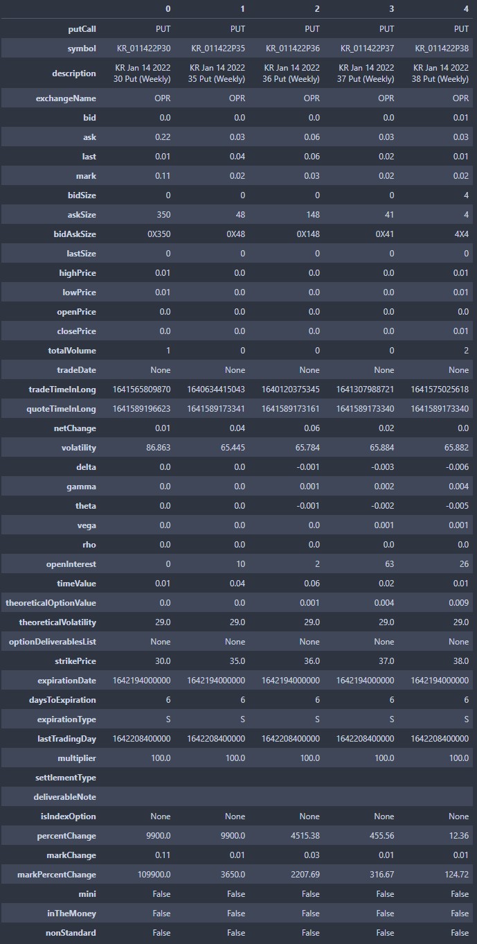
It should be clear that the entity on which we’re collecting data is a contract (defined by an expiry date and strike) at a specific time.
Data Size
We see that the data has the potential to grow in size really quickly. The sample contained 297 rows and 47 columns of data. If we narrow this down to about 30 columns and collect the data, say, every 30 minutes, that amounts to approximately 30MB per month, per ticker (estimated using CSV file size). For the small scale use case, 600MB will be added to the repository every month. For the large scale use case, this figure is a whopping 30GB. The amount of storage we need to provision depends on how much data we want to analyse at a time:
| Lookback Period | Small Scale | Large Scale |
|---|---|---|
| 12 months | 7.2GB | 360GB |
| 24 months | 14.4GB | 720GB |
| 36 months | 21.6GB | ~ 1TB |
Choosing a Database Type
I know I already revealed the chosen database (PostgreSQL) in the introduction, but I will still detail the considerations for my choice. First, we use Database Zone’s database decision matrix [8] to decide whether to use a relational (SQL) or non-relational (“NoSQL”) database.
| Requirements | Details | Small Scale | Large Scale |
|---|---|---|---|
| ACID compliance for transactions | Not processing transactions. Not essential. | Either will do. | Either will do. |
| Security and integrity | Data is simple and not PID. | Either will do. | Either will do. |
| Data structure | Structured time series that is unlikely to change. | SQL +1 | SQL +1 |
| Redundancy and data normalisation | Depends on scenario. | Not essential. Either will do. | Redundancy is essential for service continuity. NoSQL +1. |
| Entity relationships and consistency | No relationships: Data across tickers and contracts are independent. Relational databases are not necessary. | Either will do. | Either will do. |
| Complexity of queries | Simple queries. | Either will do. | NoSQL has better performance. NoSQL + 1. |
| Performance and availability | Depends on scenario. | Low performance/availability requirements. Either will do. | High performance requirements. NoSQL +1. |
| Scalability | Depends on scenario. | Difficult to scale horizontally, but given the size, it shouldn’t cost much to scale vertically by a small amount. Either will do. | Needs to scale. NoSQL + 1. |
The table above gives us the total scores below:
| Database Type | Scores - Small Scale | Scores - Large Scale |
|---|---|---|
| SQL | 8 / 8 | 4 / 8 |
| NoSQL | 7 / 8 | 7 / 8 |
Based on this criteria, a SQL database seems to be slightly more suitable for the small scale scenario because we don’t need the benefits of NoSQL databases. For the large scale scenario, a NoSQL database may be more suitable due to the need for performance, scalability and availability.
Choosing a Database Engine
So far, we’ve figured that we ought to choose a relational database for our small scale scenario, and a non-relational database for the large scale one. It’s time to select a specific database engine.
For the small scale scenario, MySQL and Postgres were 2nd and 4th in popularity by DB-Engines’ ranking [9], respectively. Both are well-established, popular, and have great community support. Although Postgres ranked lower, it has a major advantage over MySQL for our Airflow solution. Assuming the database we choose also serves as the backend for our Airflow instance, Postgres allows us to transfer a much larger amount of data between tasks (1GB) in the pipeline compared to MySQL (64kb). We will explain this in more detail in the posts to come.
Full disclosure: I’m personally more familiar with Postgres than MySQL, and I’m a big fan of pgAdmin.
For the large scale scenario, and for users who want to scale up to much more than 20 stocks, MongoDB looks like the most sensible option. The major CSPs all provide hosting services, and MongoDB itself offers a really affordable serverless solution.
But what about time series databases like InfluxDB and TimescaleDB? Aren’t we dealing with time series data? Yes, we are. However, these databases are optimised for real-time monitoring of IoT devices, which deals with large volumes of reads and writes per second. That’s overkill for our use case. Other reasons why we might want to stick to Postgres:
- It’s more popular and it’s more likely that users can get support for it
- It’s familiar: SQL
- It’s more convenient (in terms of maintenance and backups) to operate a single database
- Commercial solutions for time series databases are more costly
That said, if we were collecting data at a much higher frequency (e.g. 1-minute), it would be worth exploring time series databases.
Scaling Options
For the small scale use case, we may not need to look into scaling up our storage (36 months of 20 stocks ~ 21.6GB). But out of curiosity, I obtained quotes from database hosting services for several popular engines. We use the following assumptions:
| Requirement | Small Scale | Large Scale |
|---|---|---|
| Storage for 24 months lookback | 15GB | 720GB |
| Backup Storage | 1.5 x 15GB = 22.5GB | 1.5 x 720GB = 1TB |
| CPU | 1 x vCPU, 0.5-1GB RAM | 2 x vCPU, 8GB RAM |
| Hours Run | 13 hours per day x 6 days per week x 4+ weeks = 338 hours per month | 338 hours per month |
| Writes | 20 stocks x 2 times per hour x 13 hours per day x 21 days per month = ~11k per month | 11k x 50 = 550k per month |
| Reads | 20 stocks x 100 reads = 2000 per month | 1,000 stocks x 1,000 reads = 1,000,000 per month |
| Throughput - Writes to be completed within 5 minutes | 20 stocks x 300 rows / 5 minutes = 20 writes per second | 1,000 stocks x 300 rows / 5 minutes = 1,000 writes per second |
The cost table:
| Type | Service | Small Scale | Large Scale | Remarks |
|---|---|---|---|---|
| SQL | AWS RDS for PostgreSQL/MySQL [10] | SGD16.69 | SGD377.07 | - |
| SQL | Azure Database for PostgreSQL/MySQL [11] | SGD17.65 | SGD321.71 | - |
| SQL | GCP Cloud SQL for PostgreSQL/MySQL [12] | SGD12.71 | SGD350.21 | - |
| NoSQL | MongoDB Atlas - Serverless [13] | SGD5.52 | SGD246.04 | New release (Jul 21) |
| NoSQL | MongoDB Atlas - AWS [14] | SGD45.96 | SGD753.67 | - |
| NoSQL | MongoDB Atlas - Azure [15] | SGD50.55 | SGD914.51 | - |
| NoSQL | MongoDB Atlas - GCP [16] | SGD55.15 | SGD827.20 | - |
It’s a relief to see that we can host a relational database that meets our needs for under SGD20 per month. It’s also interesting to see that MongoDB currently offers a serverless service that beats pretty much all the other solutions in price. Since it is a new service offering, we should keep an eye on it.
Having made our choice, we can proceed to set up Postgres. If you’re on Linux and have Ubuntu 20.04 installed, we won’t need to do a lot to get Postgres running because Ubuntu 20.04 comes with Postgres packages by default. To install it, all you need to run in bash is:
apt-get install postgresql
Postgres associates its roles with a matching system account. Hence, next, we need to log in to the postgres account on our system. This starts the server, and gives us access to the default Postgres database role. Use the commands below in bash to switch to the postgres system account and open the Postgres terminal:
# Switch account and start server
sudo -i -u postgres

# Open Postgres terminal
psql
Next, we change our password. Note this down because we’ll need it when loading the data in.
-- Change password (optional)
ALTER USER postgres PASSWORD 'new_password';
Database Structure
Let’s think about the use case again. In running backtests, we know that the options data for each ticker would probably be fused with the corresponding stock data and technical indicators. It is unlikely that we would need data for different tickers in the same table. In fact, dumping data for multiple tickers into the same table would only slow down our queries. Hence, we create one table per ticker.
To separate the options data from Airflow’s system data, we create a new database within Postgres:
-- Create database
CREATE DATABASE optionsdata;

-- Verify that database is created
\l
Table Structure
With our database up and running, we define what each table should look like. From our inspection of the data earlier, we know that the entity we are collecting data on is a contract (defined by an expiry date and strike) at a specific time. The available attributes of interest are:
- Metadata: putCall, symbol, description, quoteTimeInLong (as unix timestamp)
- Contract info: openInterest, timeValue, theoreticalOptionalValue, strikePrice, expirationDate (as unix timestamp), daysToExpiration, volatility
- Trade data: bid, ask, last, bidSize, askSize, lastSize, highPrice, lowPrice, openPrice, closePrice, totalVolume
- Greeks: delta, gamma, theta, vega, rho
Next, we connect to the newly-created database and create a new table based on the data formats that we identified from earlier on:
-- Connect to optionsdata
\c optionsdata

-- Create table
CREATE TABLE IF NOT EXISTS fb (
    put_call VARCHAR(5) NOT NULL,
    symbol VARCHAR(32) NOT NULL,
    description VARCHAR(64) NOT NULL,
    bid DOUBLE PRECISION,
    ask DOUBLE PRECISION,
    last DOUBLE PRECISION,
    bid_size INTEGER,
    ask_size INTEGER,
    last_size INTEGER,
    high_price DOUBLE PRECISION,
    low_price DOUBLE PRECISION,
    open_price DOUBLE PRECISION,
    close_price DOUBLE PRECISION,
    total_volume INTEGER,
    quote_time BIGINT,
    volatility DOUBLE PRECISION,
    delta DOUBLE PRECISION,
    gamma DOUBLE PRECISION,
    theta DOUBLE PRECISION,
    vega DOUBLE PRECISION,
    rho DOUBLE PRECISION,
    open_interest INTEGER,
    time_value DOUBLE PRECISION,
    theoretical_value DOUBLE PRECISION,
    strike_price DOUBLE PRECISION,
    expiration_date BIGINT,
    dte INTEGER,
    PRIMARY KEY (symbol, quote_time)
);

-- Verify that table was created
\dt

-- Exit Postgres terminal
\q
The main data types are VARCHAR(N), INTEGER, DOUBLE PRECISION, and BIGINT (for unix timestamps - quote time and expiration date only). To uniquely identify each row based on the logical entity (contract with a specific expiry date and strike at a specific time), we create a composite primary key comprising the strike’s symbol (i.e. a specific strike for a specific contract) and the quote time.
Summary
In this post, we examined the different requirements for a small scale use case (20 stocks) and a large scale use case (1,000 stocks), decided on using PostgreSQL as our database system, and set up a database and table in PostgreSQL. In the next post, we’ll move on to developing the code for an ETL pipeline.
Credits for image: Kevin Ku on Unsplash
References
- E. Kleppen, Collecting Stock and Options Data Easily using Python and Ally Financial API - 3 Example Queries (2020), TowardsDataScience
- Blackarbs, Aggregating Free Options Data with Python (2016), Blackarbs.com
- H. Sauers, How I get options data for free (2019), freeCodeCamp
- A. Treadway, How To Get Options Data with Python (2019), TheAutomatic.net
- T. Lian, Webscrapping Options Data with Python and YFinance (2020), Medium
- CodeArmo, Getting Options Data from Yahoo Finance with Pandas (2020), CodeArmo
- R. Aroussi, Downloading option chain and fundamental using Python (2019), aroussi.com
- S. Tol, SQL vs NoSQL and SQL to NoSQL Migration (2021), DZone
- DB-Engines, DB-Engines Ranking (2022), DB-Engines
- Amazon Web Services, AWS Pricing Calculator
- Microsoft Azure, Pricing Calculator
- Google, Google Cloud Pricing Calculator
- MongoDB, MongoDB Pricing
- Ibid.
- Ibid.
- Ibid.